
GenBank Flat File Visualization
In this tutorial we’ll show how to create a simple Circleator figure for a genome sequence–and any associated annotation–in GenBank flat file format. We’ll look at two examples, one of which is a completed microbial genome sequence, and one of which is an unfinished draft genome sequence. Before proceeding with the tutorial, please make sure that you have Circleator installed as described in the Circleator Installation Guide.
Outline
-
Example 1: Completed Genome of Haemophilus influenzae Rd KW20
-
Example 2: Draft Genome Sequence of Propionibacterium acnes HL005PA3
Example 1: Completed Genome of Haemophilus influenzae Rd KW20
Download the GenBank flat file
The GenBank accession number for the Haemophilus influenzae Rd KW20 genome sequence is L42023.1. For convenience we’ve downloaded the corresponding GenBank flat file and placed a copy on the same web server as the Circleator tutorials (see below). Download this .gb file by right-clicking on the link below and selecting “Save link as” or “Save as”. Save the file somewhere accessible because we’ll be using it as one of the inputs to Circleator:
If you want to download a different genomic sequence entry you can do so by using NCBI’s GenBank web site, as described here.
Download the Circleator configuration file
Here is a very simple Circleator configuration file. Download it by right-clicking on the following link and selecting “Save link as” or “Save as”:
Take a look at the content of this file e.g., by using the cat command in Linux/Unix:
$ cat genes-only.txt

coords
small-cgap
genes
Each of the lines in this file–and in any Circleator configuration file–corresponds to exactly one circular “track” and, by default, the first track listed in the file (i.e., coords in this case) is the outermost one in the figure. Each successive track/line in the configuration file is placed immediately inside the track before, until the available space in the circle has been exhausted.
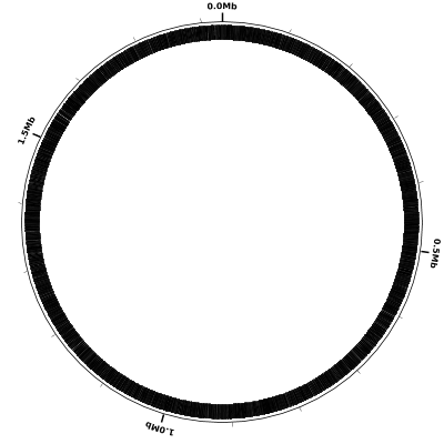
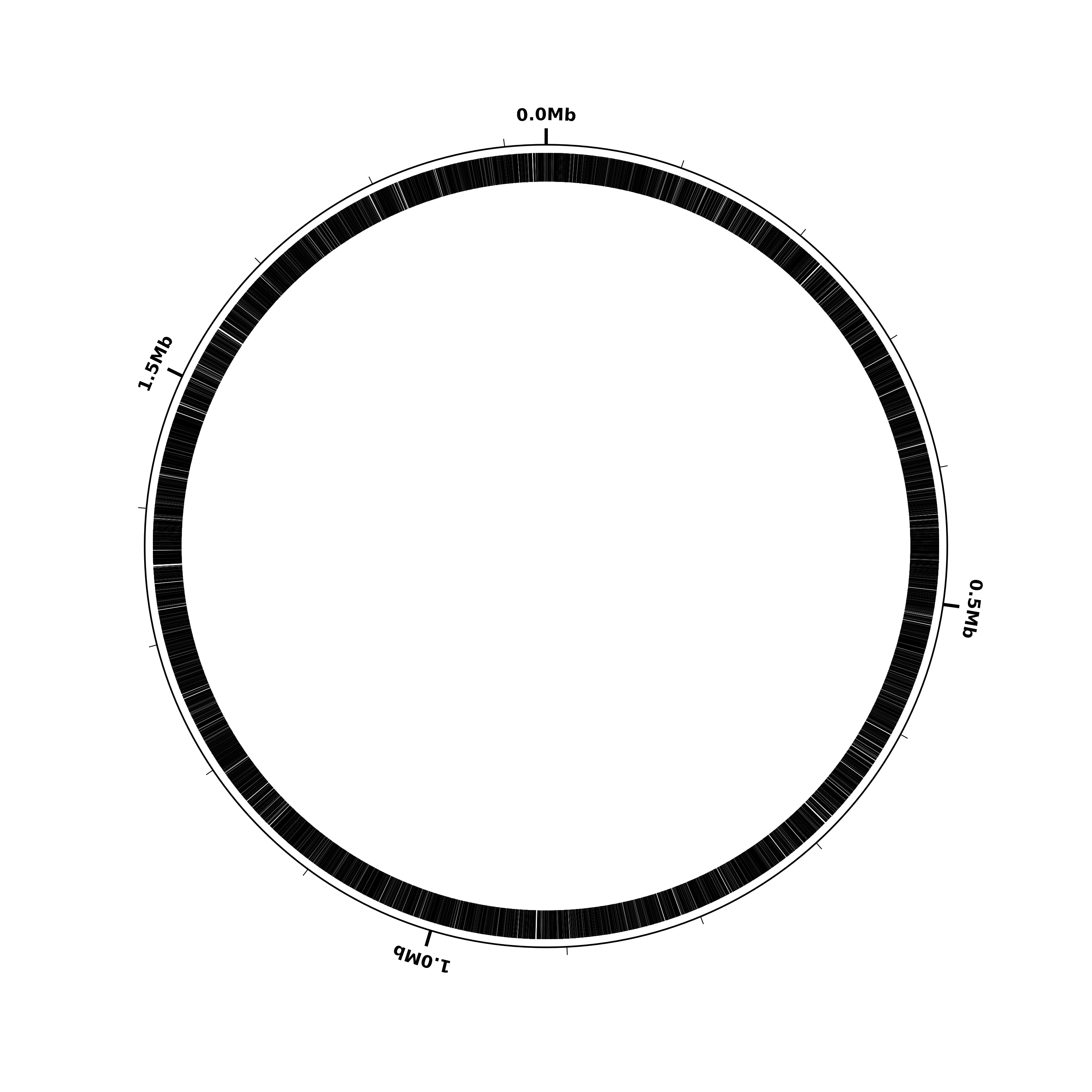
In this particular configuration file each of the lines contains a single predefined track name (coords, small-cgap, and genes). These predefined tracks display the following:
- coords - a circle representing the 1.83 Mb H. influenzae Rd KW20 genome, with:
- a tick mark drawn every 100 kb
- a label (e.g., 0.0Mb, 0.5Mb) drawn every 0.5 Mb
- small-cgap - a small (circular) gap between the previous track and the next
- genes - a curved black rectangle at the location of each gene feature in the input GenBank file.
A more complete list of the predefined track types can be found on the predefined track types page. There is also a page that describes the configuration file format in detail.
Run Circleator
Now that we have both an input annotation file and a Circleator configuration file, all that remains is to run Circleator, like so:
$ circleator --data=L42023.1.gb --config=genes-only.txt --pad=100 > hinf-genes-only.svg
Note that Circleator prints its (SVG) output to stdout, so we must use the shell redirection character (“>”) to place it into a file of our choosing (hinf-genes-only.svg) Also, if the Circleator output includes a warning about “Unrecognized DBSOURCE data” this may be ignored: it’s a warning generated by certain versions of BioPerl but it should not affect the results. Here’s what the Circleator output might look like on the terminal after running the above command:
INFO - started drawing figure using genes-only.txt
INFO - reading from annot_file=./L42023.1.gb, seq_file=, with seqlen=
--------------------- WARNING ---------------------
MSG: Unrecognized DBSOURCE data: BioProject: PRJNA219
---------------------------------------------------
INFO - L42023: 3521 feature(s) and 1830138 bp of sequence
INFO - read 1 contig(s) from 1 input annotation and/or sequence file(s)
INFO - finished drawing figure using genes-only.txt
Convert the figure from SVG to PNG
SVG (Scalable Vector Graphics) format is a vector-based graphics format, meaning that the image is composed of geometrical primitives like lines, circles, and arcs. Magnifying a vector-based image does not result in any loss of image quality, making SVG well-suited for publication purposes, in which a very high-quality image is desirable. Image formats like JPEG and PNG are “raster” (pixel-based) formats, in which the image is made up of many colored rectangular blocks (the pixels), like an LCD screen. Some programs, like Adobe Illustrator, can view and manipulate SVG images directly. For many purposes, however, it is convenient to have a pixel-based image format. The rasterize-svg utility, distributed with Circleator, makes use of the Apache Batik package to convert SVG images to either PNG, JPEG, or PDF. (PDF is also a vector-based format, although both it and SVG may contain pixel-based images.) Converting our SVG-format figure to a PNG image will take a few seconds, and can be done with the following command:
rasterize-svg hinf-genes-only.svg png 3000 3000
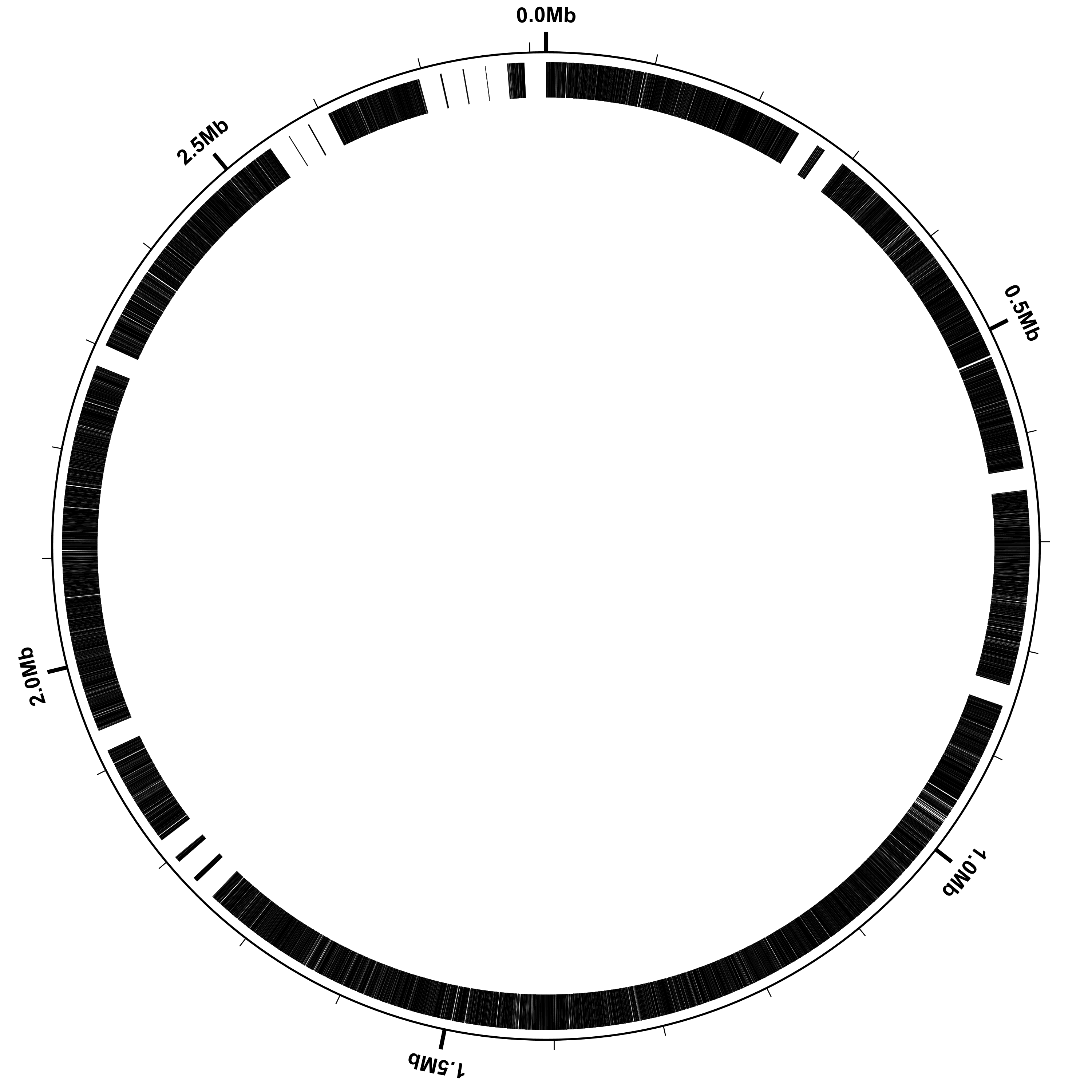
When rasterizing SVG it is necessary to specify the size of the resulting raster image, and the “3000 3000” indicate that the image should be 3000 pixels wide by 3000 pixels high. Here is the resulting PNG image:
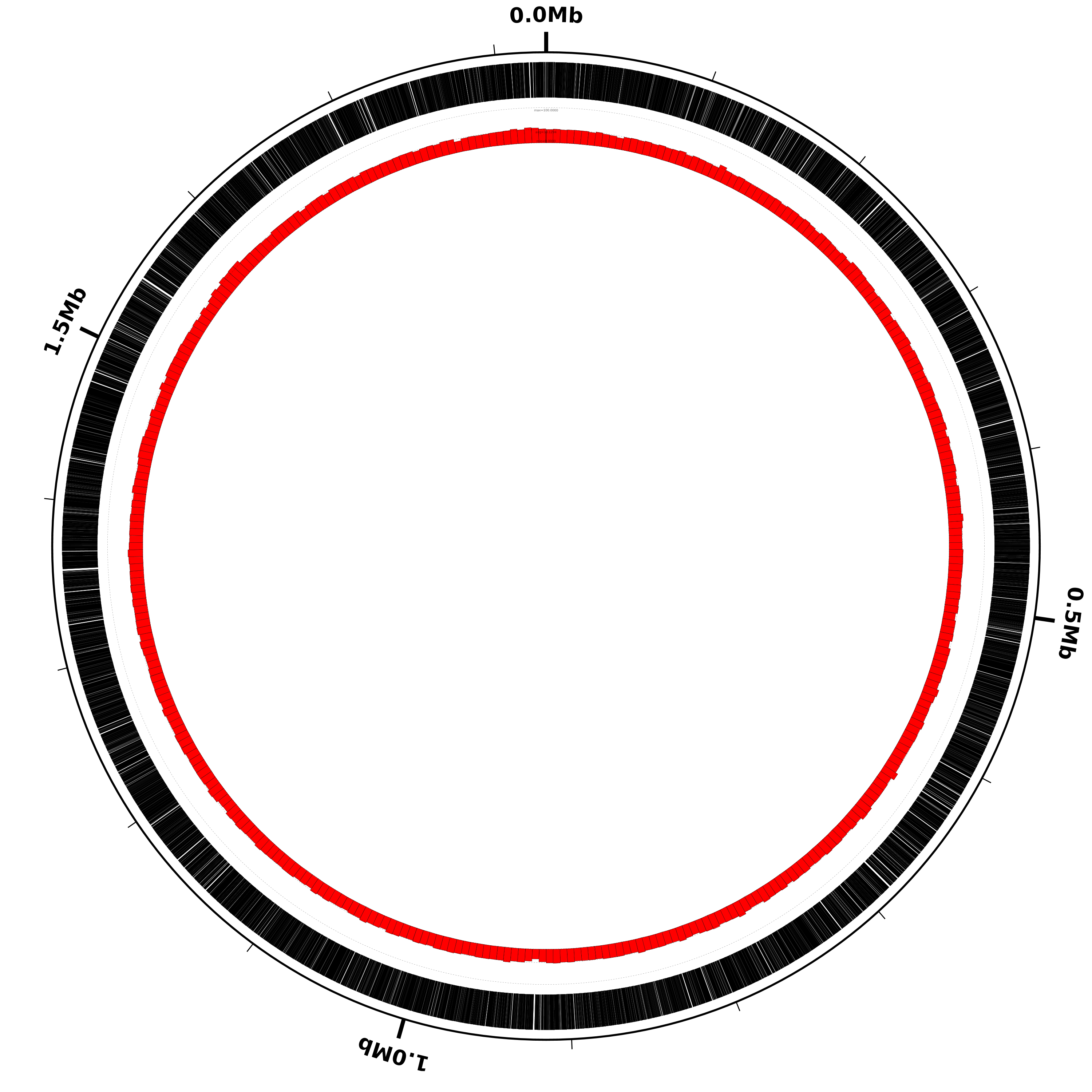
Add a percent GC-content plot
Now let’s display a simple quantity computed directly from the DNA sequence, namely the percent GC-content. Percent GC-content is typically plotted using a sliding window and by default Circleator uses nonoverlapping windows. Here is our sample configuration file (genes-and-percentGC-1.txt) with another small circular gap (small-cgap) and a default percent GC plot (%GC0-100):
coords
small-cgap
genes
small-cgap
%GC0-100
Run Circleator as before, passing it both the configuration file and the GenBank flat file and directing the output into a .svg file, and then rasterize the SVG file:
circleator --data=L42023.1.gb --config=genes-and-percentGC-1.txt --pad=100 > hinf-genes-pctgc-1.svg
rasterize-svg hinf-genes-pctgc-1.svg png 3000 3000
Here is the resulting figure:
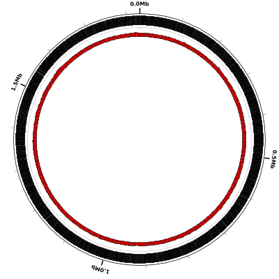
The percent GC plot doesn’t appear to be very informative, although if
you look at one of the full-size figures you can see that the percent
GC content stays right around the average value (38.1%) pretty much
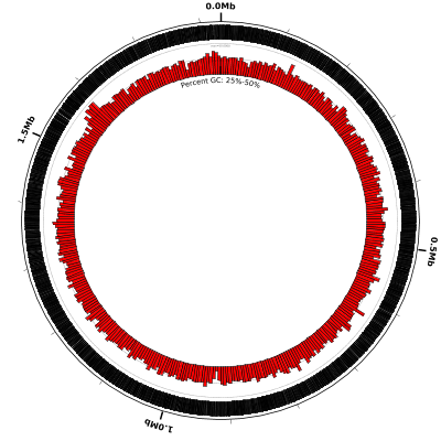
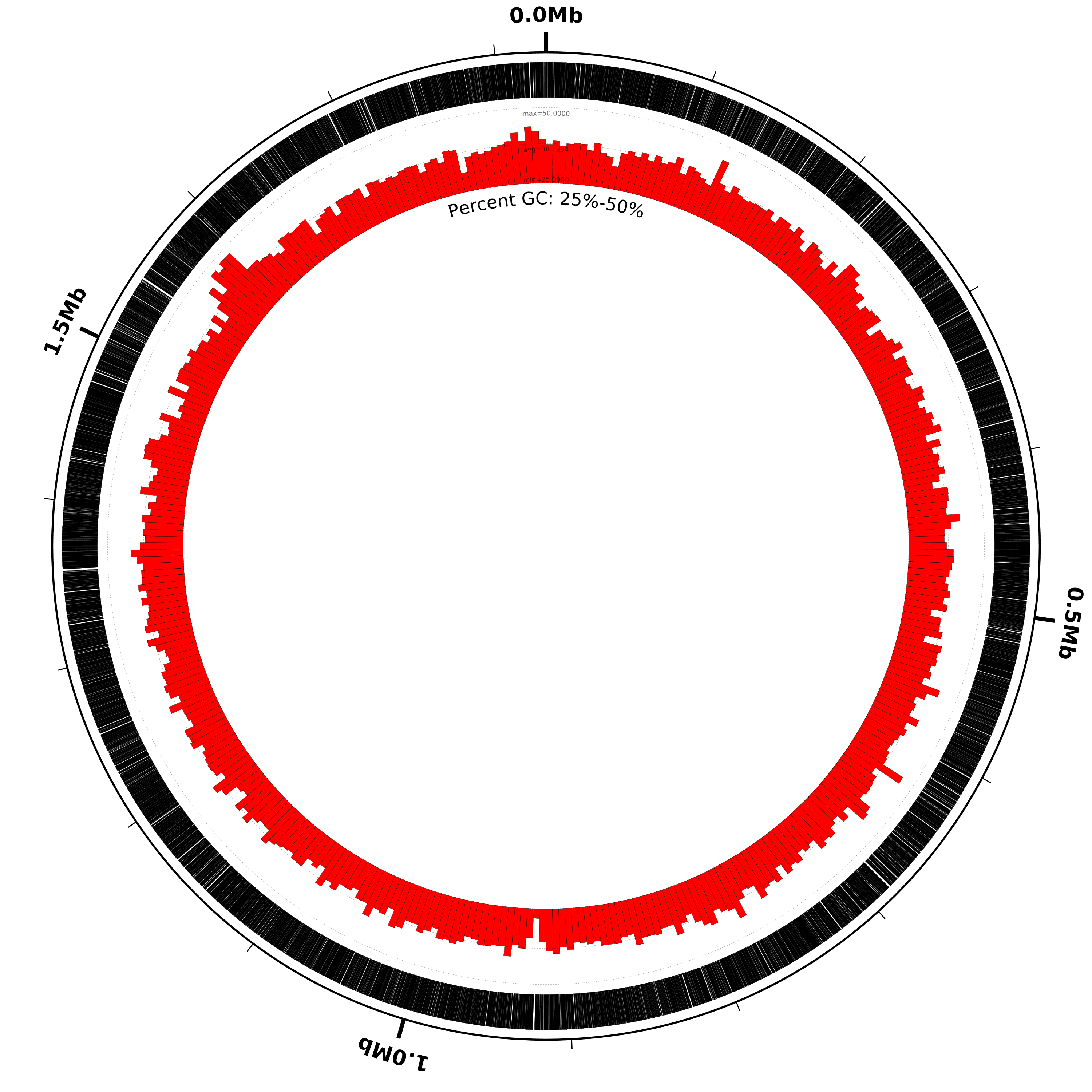
throughout the entire genome. In fact, if we run Circleator with more
verbose debugging enabled (--debug=misc or --debug=all) then it
will tell us the observed minimum and maximum values for each of the
graphs it draws, like so:
DEBUG - graph data observed min=28.18, max=47.72, avg=38.129371717411, nvals=367, g_baseline=range_min, g_min=0, g_max=100
This tells us that although the %GC0-100 track is drawn with range 0-100 (g_min=0, g_max=100)
the actual observed minimum value (for the given default window size) is 28.18 and
the observed maximum value is 47.72. We can modify the percent-GC graph to
show more detail by decreasing the range accordingly, perhaps to 0-50
or even 25-50. We can also increase the height of the graph to show more
detail, as in the following example configuration file:
coords
small-cgap
genes
small-cgap
# decrease graph_max from 100 to 50, increase graph_min to 25
# and increase heightf from 0.07 to 0.15:
%GC0-100 graph_max=50,graph_min=25,heightf=0.15
# add a label to make it clear what's going on:
medium-label label-text=Percent GC: 25%-50%
Run Circleator and rasterize the resulting SVG file:
circleator --data=L42023.1.gb --config=genes-and-percentGC-2.txt --pad=100 --debug=misc > hinf-genes-pctgc-2.svg
rasterize-svg hinf-genes-pctgc-2.svg png 3000 3000
And the figure now looks like this:
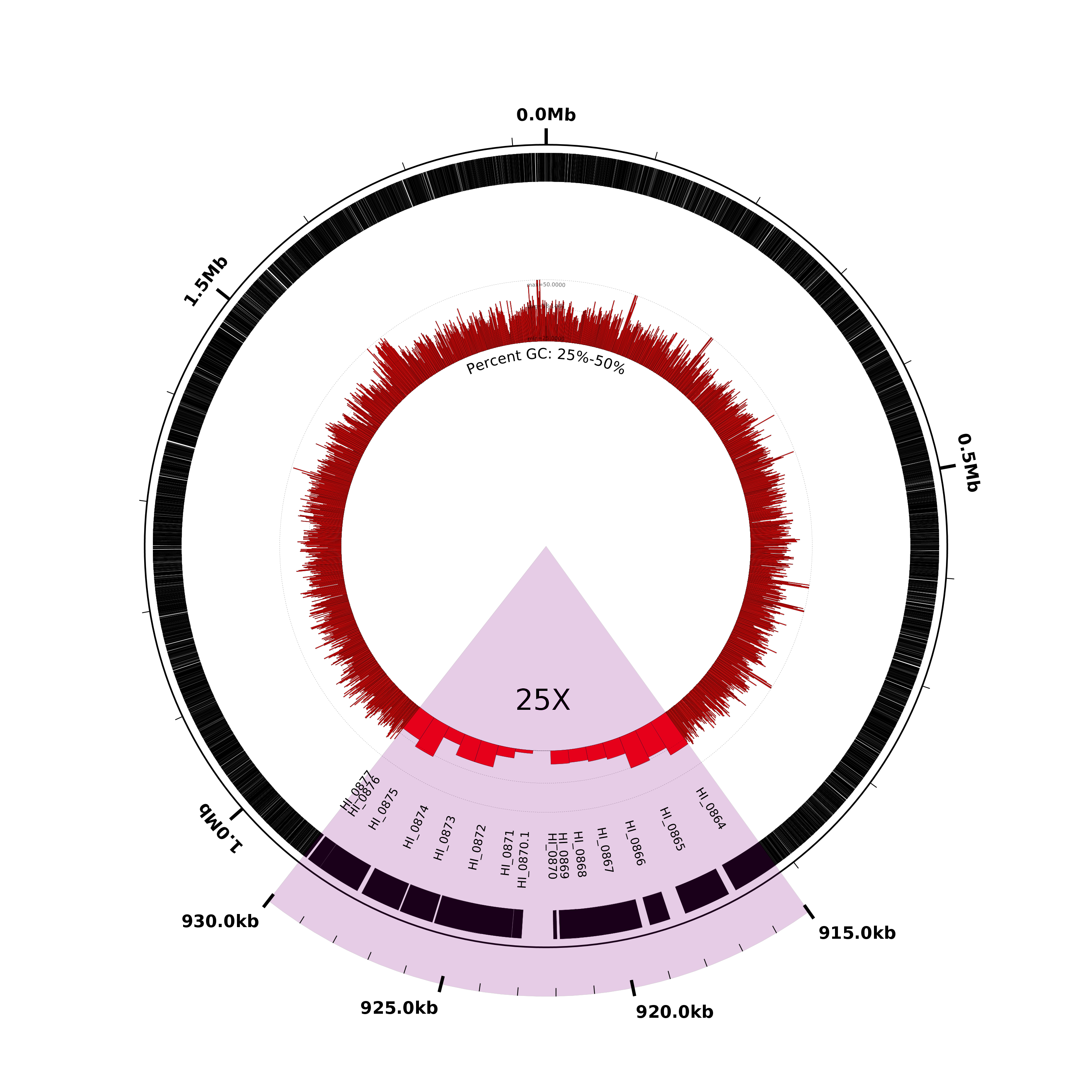
Magnify and highlight a region of interest
By default Circleator draws each genomic sequence to scale, but the scale can be changed in order to show greater detail in regions of interest (at the expense of having a figure that is no longer drawn to scale.) In this next figure we’ll use the scaled-segment-list track type to modify the scale, expanding a single region from 910-930kb by a factor of 25. Circleator will automatically compress the scale for the rest of the figure to compensate for the change. Let’s run Circleator and rasterize the resulting SVG file, and then talk about what changes were made to the configuration file:
circleator --data=L42023.1.gb --config=explore-region-1.txt --pad=100 --debug=misc > explore-region-1.svg
rasterize-svg explore-region-1.svg 3000 3000
Here’s what the result should look like. Notice that the highlighted region at the bottom (highlighted in pink and labeled “25X”) has been expanded compared to the rest of the figure:
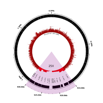
The following two lines in the configuration file effect the change of scale:
# zoom in 25X on the region from 910-930kb
new r1 load user-feat-fmin=915000,user-feat-fmax=930000,user-feat-type=roi
new ss1 scaled-segment-list scale=25,feat-type=roi
Note that any changes in scale will affect only the subsequent lines in the configuration file, which is why we’ve placed the scale-changing lines above at the very beginning of the file. Note also that we’ve broken the change of scale into two parts: in the first line we define a new user-defined feature, with position 910-930kb and type “roi”:
new r1 load user-feat-fmin=915000,user-feat-fmax=930000,user-feat-type=roi
In the second line, we scale by a factor of 25X all those regions covered by features of type “roi” i.e., the single region we just created:
new ss1 scaled-segment-list scale=25,feat-type=roi
The next several lines of the configuration file are identical to those from the previous example and then the final four lines add some color and labels to the expanded region:
# highlight and label the zoomed region
new h1 rectangle innerf=0,outerf=1.1,opacity=0.2,color1=purple,feat-type=roi
coords outerf=1.1,fmin=915000,fmax=930000,tick-interval=1000,label-interval=5000,no-circle=1,label-units=kb,label-type=horizontal
large-label innerf=0.4,label-text=25X,label-position=922500,label-type=horizontal
medium-label innerf=0.7,label-type=spoke,label-function=locus,overlapping-feat-type=roi,feat-type=gene,packer=none,heightf=0.04
Let’s look at each of these four lines in detail:
new h1 rectangle innerf=0,outerf=1.1,opacity=0.2,color1=purple,feat-type=roi
The first field in any line is mandatory and must be either the name of a predefined track or the keyword new otherwise (as in this case.) The second optional field assigns a name to the track, h1 in this case. Assigning a unique name is recommended so that other tracks may refer unambiguously to this one if needed. The third field specifies the “glyph” or underlying graphical primitive to use, in this case rectangle, the curved rectangle glyph that Circleator uses for many of its tracks. The final field specifies the track options, separated by commas. The options in this line are:
- innerf=0 : the inner “edge” of the track is the very center of the circle
- outerf=1.1 : the outer edge of the track is 110% of the circle’s radius
- opacity=0.2 : the track is 80% transparent
- color=purple : the track is shaded purple (light purple because of the opacity setting)
-
feat-type=roi : only features of type “roi” (i.e., our single region of interest) are drawn
coords outerf=1.1,fmin=915000,fmax=930000,tick-interval=1000,label-interval=5000,no-circle=1,label-units=kb,label-type=horizontal
The second line (above) uses the coords predefined track type, which draws a circle and labels it with coordinate positions. We already have a coords track in the configuration file, which draws a full circle and then places a label every 0.5Mb. This coords track, on the other hand, covers only the region of interest (fmin=915000,fmax=930000) and does not draw a circle, only tick marks and labels (no-circle=1)
large-label innerf=0.4,label-text=25X,label-position=922500,label-type=horizontal
The third line (above) uses the large-label predefined track type to label the expanded region with a large “25X” label. Note that the label has been positioned manually at the center of the region (label-position=922500) and that a “horizontal” label type has been chosen (as opposed to the default, which is to draw the label on an arc of the circle.)
medium-label innerf=0.7,label-type=spoke,label-function=locus,overlapping-feat-type=roi,feat-type=gene,packer=none,heightf=0.04
The fourth line (above) uses the medium-label predefined track type to label each gene (feat-type=gene) with its locus id (label-function=locus). The “spoke” label-type is used in this case to minimize the amount of space (around the circle) taken up by each label. Finally, and crucially, note that the overlapping-feat-type=roi option restricts this labeling so that only gene features that also happen to overlap with the region of interest are labeled in this manner. Without this option all of the genes would be labeled, and the labels for those not in the expanded region would be hard or impossible to read because they’d be packed too densely.
Example 2: Draft Genome Sequence of Propionibacterium acnes HL005PA3
Download the GenBank flat file(s)
Unlike the Haemophilus influenzae sequence, which is a single finished sequence, the Propionibacterium acnes sequence is a high-quality draft that comprises 17 separate scaffolds. Each of the 17 scaffold sequences is a separate GenBank entry, and we could download them as separate files, but the simplest approach is to download a single GenBank flat file that contains all 17 sequences and their associated annotation. For convenience we’ve placed a copy of this GenBank file at the following location. Download it by right-clicking on the link below and selecting “Save link as” or “Save as”. Save the file somewhere accessible because we’ll be using it as one of the inputs to Circleator:
This file can also be downloaded from the GenBank web site with the following sequence of steps:
- Go to http://www.ncbi.nlm.nih.gov/genbank and search “All Databases” for “Propionibacterium acnes HL005PA3”
- Click on the result row for “Assembly”, to get to this page.
- Click on the “WGS Project” link, to get to this page.
- Click on the “WGS_SCAFLD” link at the bottom (“GL383461-GL383477”) to get to this page.
- Use the “Send to:” pull-down menu at the top right to select “File” and “GenBank (full)” for the format
- Click on “Create File”
- Rename the downloaded file from “sequence.gb” to “GL383461-GL383477.gb”
Download the Circleator configuration file
We’ll start with the same Circleator configuration file that was used in Example 1. If you have not already downloaded it, you may do so by right-clicking on the following link and selecting “Save link as” or “Save as”:
Recall that this 3-line configuration file displays the coordinate system labels and the gene features, and nothing else.
Run Circleator
Now that we have both an input annotation file and a Circleator configuration file, all that remains is to run Circleator, like so:
$ circleator --data=GL383461-GL383477.gb --config=genes-only.txt --pad=100 > pa-genes-only.svg
Notice that the Circleator output is slightly more verbose than in Example 1, because for each of the contigs and/or scaffolds in the input file it prints a line giving the sequence length and feature count:
INFO - started drawing figure using genes-only.txt
INFO - reading from annot_file=./GL383461-GL383477.gb, seq_file=, with seqlen=
INFO - GL383461: 493 feature(s) and 246684 bp of sequence
INFO - GL383462: 19 feature(s) and 8634 bp of sequence
INFO - GL383463: 649 feature(s) and 336359 bp of sequence
INFO - GL383464: 400 feature(s) and 182889 bp of sequence
INFO - GL383465: 1862 feature(s) and 893497 bp of sequence
INFO - GL383466: 5 feature(s) and 4650 bp of sequence
INFO - GL383467: 9 feature(s) and 5617 bp of sequence
INFO - GL383468: 219 feature(s) and 97238 bp of sequence
INFO - GL383469: 766 feature(s) and 347101 bp of sequence
INFO - GL383470: 518 feature(s) and 240912 bp of sequence
INFO - GL383471: 5 feature(s) and 778 bp of sequence
INFO - GL383472: 3 feature(s) and 1168 bp of sequence
INFO - GL383473: 186 feature(s) and 90326 bp of sequence
INFO - GL383474: 3 feature(s) and 1380 bp of sequence
INFO - GL383475: 3 feature(s) and 889 bp of sequence
INFO - GL383476: 5 feature(s) and 616 bp of sequence
INFO - GL383477: 37 feature(s) and 16090 bp of sequence
INFO - read 17 contig(s) from 1 input annotation and/or sequence file(s)
INFO - finished drawing figure using genes-only.txt
Convert the figure from SVG to PNG
As in example 1, let’s convert the SVG image to PNG:
$ rasterize-svg pa-genes-only.svg png 3000 3000
Here is the result:

genes-only.txt:
coords
small-cgap
genes
Note that in this figure we have several gene-free regions, which did not appear in example 1. The reason for this is that we have 17 scaffolds and, by default, Circleator places a 20 kb gap between each pair of adjacent scaffolds or contigs. Also by default, Circleator draws the contigs/scaffolds in the same order (clockwise, starting at the origin) that they appear in the input GenBank file.
Show the scaffold locations
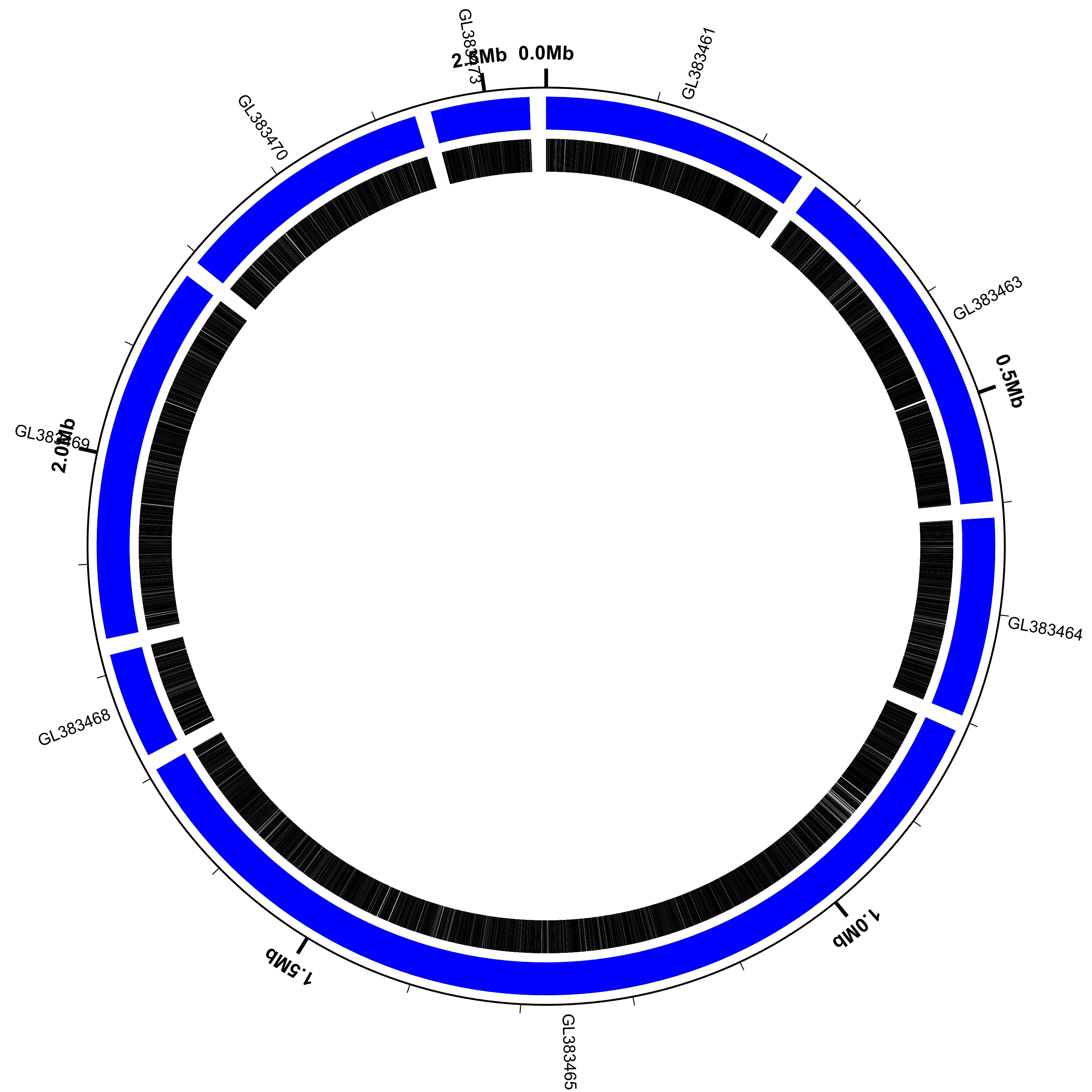
Let’s modify the configuration file slightly so that we can see the scaffold locations and accession numbers in the figure. Here’s the updated configuration file:
Now run Circleator and convert the SVG figure to PNG format. Note that
we’re increasing the --pad amount from 100 to 200 to make room for the
scaffold labels around the outside of the circle:
$ circleator --data=GL383461-GL383477.gb --config=scaffolds-and-genes.txt --pad=200 > pa-scaffolds-and-genes.svg
$ rasterize-svg pa-scaffolds-and-genes.svg png 3000 3000
(data: GL383461-GL383477.gb config: scaffolds-and-genes.txt, full size PNG | SVG)
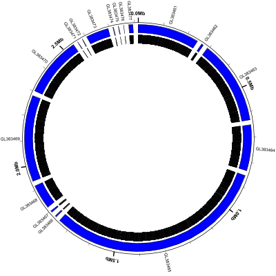
scaffolds-and-genes.txt:
coords
small-cgap
contigs c1
small-cgap
genes
medium-label innerf=1.0,label-function=primary_id,feat-track=c1,label-type=spoke,packer=none
Note that:
- the
contigspredefined track type displays each contig or scaffold as a blue curved rectangle - we’ve given the
contigstrack a name (c1) so we can refer to it later - the
medium-labeltrack at the end labels each scaffold with its primary_id/accession number label-type=spokeis used to prevent adjacent labels from overlappingpacker=nonetells Circleator not to try to move labels around to avoid collisions- some of the scaffolds are very small (616 bp according to the circleator output)
Filter out the short sequences
Circleator has a couple of command-line options that affect the handling of multi-sequence
input data. One is --contig_gap_size, which can be used to change the default gap placed
between adjacent contigs/scaffolds (20kb by default). Another is --contig_min_size, which
specifies a minimum contig/scaffold length (in bp). Sequences that are shorter than this
will be excluded from the display. Let’s use these two options, along with the same
configuration file as the previous example, to change the figure a bit:
$ circleator --data=GL383461-GL383477.gb --config=scaffolds-and-genes.txt --pad=200 --contig_min_size=50000 --contig_gap_size=15000 > pa-no-short-scaffolds.svg
$ rasterize-svg pa-no-short-scaffolds.svg png 3000 3000
Circleator reports that only 8 of the 17 scaffolds are 50kb or longer:
INFO - started drawing figure using scaffolds-and-genes.txt
INFO - reading from annot_file=./GL383461-GL383477.gb, seq_file=, with seqlen=
INFO - GL383461: 493 feature(s) and 246684 bp of sequence
INFO - GL383463: 649 feature(s) and 336359 bp of sequence
INFO - GL383464: 400 feature(s) and 182889 bp of sequence
INFO - GL383465: 1862 feature(s) and 893497 bp of sequence
INFO - GL383468: 219 feature(s) and 97238 bp of sequence
INFO - GL383469: 766 feature(s) and 347101 bp of sequence
INFO - GL383470: 518 feature(s) and 240912 bp of sequence
INFO - GL383473: 186 feature(s) and 90326 bp of sequence
INFO - read 8 contig(s) from 1 input annotation and/or sequence file(s)
INFO - finished drawing figure using scaffolds-and-genes.txt
(data: GL383461-GL383477.gb config: scaffolds-and-genes.txt, full size PNG | SVG)
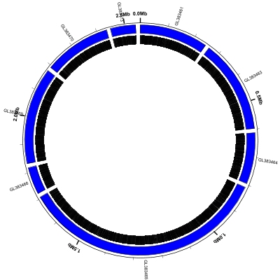
Note that:
- the coordinate labels (
coords) around the outside of the circle include the gaps as well as the scaffold sequences - some of the scaffold labels are colliding with the coordinate labels
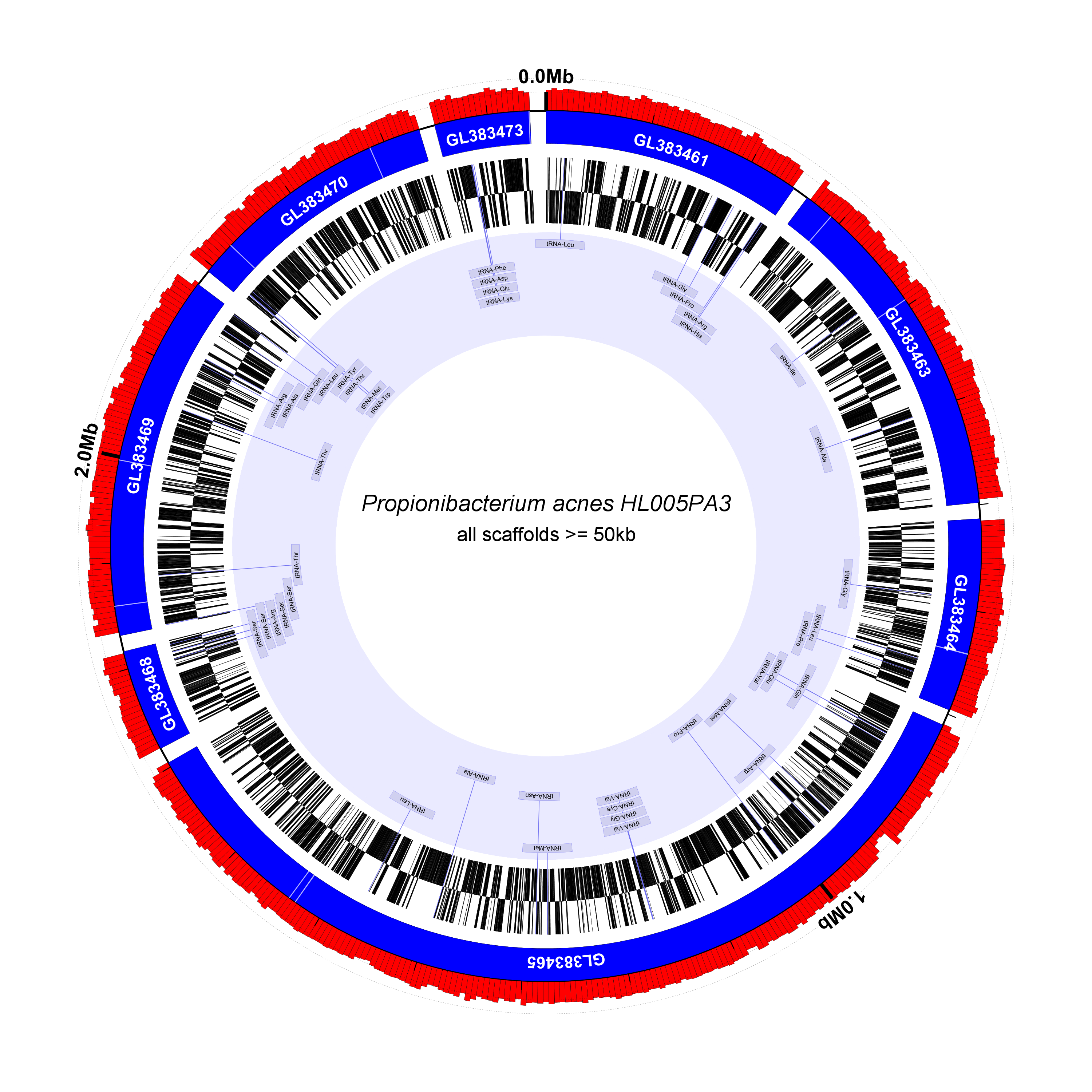
Add some flair
Now let’s make the figure a little more interesting by adding some tracks and, since all of the scaffolds are now relatively long, overlaying the scaffold id directly on the curved blue scaffold rectangles. Here’s the updated configuration file:
$ circleator --data=GL383461-GL383477.gb --config=scaffolds-and-genes-plus.txt --pad=200 --contig_min_size=50000 --contig_gap_size=15000 > pa-no-short-scaffolds-plus.svg
$ rasterize-svg pa-no-short-scaffolds-plus.svg png 3000 3000
(data: GL383461-GL383477.gb config: scaffolds-and-genes-plus.txt, full size PNG | SVG)
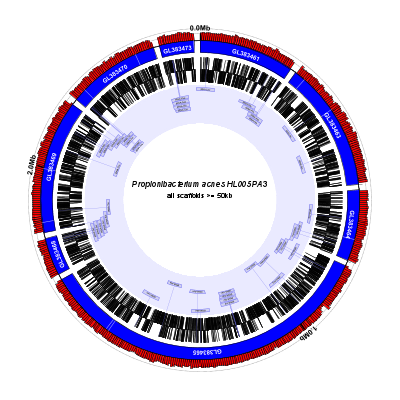
scaffolds-and-genes-plus.txt:
# percent-GC graph with coordinates overlaid
%GC0-100 graph-min=40,graph-max=70,no-labels=1
coords label-interval=1000000,innerf=same

contigs c1
# show assembly gaps as light lines on the blue scaffolds
new ag rectangle innerf=same,outerf=same,feat-type=assembly_gap,color1=white,color2=white,stroke-width=2.5,opacity=0.7
# label each scaffold with its accession number
medium-label innerf=same+0.01,label-function=primary_id,feat-track=c1,text-color=white,packer=none,font-weight=bold
tiny-cgap

# invisible tRNAs
small-cgap
tRNAs trnas heightf=0.01,color1=none,color2=none

genes-fwd
genes-rev
small-cgap

# link back to invisible tRNAs from a few tracks before
new r1 rectangle heightf=0.01,color1=#eaeaff,color2=#eaeaff
new r2 rectangle heightf=0.2,color1=#eaeaff,color2=#eaeaff
large-label heightf=0.2,outerf=same,feat-track=trnas,style=signpost,label-function=product,draw-link=1,color1=#d0d0f0,color2=#7070f0,link-color=#7070f0,stroke-width=1.5,font-width-frac=3.5
new r3 rectangle heightf=0.01,color1=#eaeaff,color2=#eaeaff

# figure caption
small-cgap
new fc1 label 0.07 innerf=0.075,label-text=Propionibacterium acnes HL005PA3,font-style=italic,label-type=horizontal
new fc2 label 0.06 innerf=0.01,label-text=all scaffolds >= 50kb,label-type=horizontal
There’s a lot going on here, so let’s take it line-by-line. Note that ines that start with “#” are comments and are ignored by Circleator:
# percent-GC graph with coordinates overlaid
We’ve changed the percent-GC graph range from 0-100 to 40-70. This is
because the artificial 15 kb gaps between the scaffolds are runs of
“N”s, which have 0% GC-content, and without these gap regions the
actual minimum %GC would be significantly higher (and would depend on
the nonoverlapping graph window size, which is 5 kb by deafult.)
Setting no-labels=1 prevents the min/max labels on the graph from
overlapping the “0.0 Mb” coordinate label:
%GC0-100 graph-min=40,graph-max=70,no-labels=1
Since the %GC graph comes before the coords track it is drawn underneath it. This is why
both tracks are visible even though the opacity option was not used. Note that we’ve
changed the label-interval to 1 Mb (to prevent the “2.5 Mb” label from running into the
“0 Mb” label.) and have set innerf=same, which means that the inner edge of this track
(coords) should be set to the same value as the inner edge of the preceding track (the
percent-GC graph). This forces the two to overlap:
coords label-interval=1000000,innerf=same
The contigs appear as blue rectangles, as before:
contigs c1
The input GenBank file contains some features of type “assembly_gap”,
to indicate the location of unclosed gaps in the scaffold
sequences. Here we draw them as slightly transparent (opacity=0.7)
white rectangles (color1=white,color2=white) overlaid on the
preceding track (outerf=same,innerf=same). Setting
feat-type=assembly_gap ensures that only features of type
“assembly_gap” will be highlighted in this manner. Finally, since the
assembly gaps are all very small with respect to the total sequence
length, we’ll draw them slightly larger than they actually are in
order to ensure that they’re visible (stroke-width=2.5). Note that
stroke-width is a CSS property that’s used in SVG to specify how
wide lines should be drawn. The rectangle glyph is a curved
rectangle with both a border (whose thickness is controlled by the
stroke-width) and also a filled interior. The two color options
(color1 and color2) determine what color to draw the border lines
and fill the interior:
# show assembly gaps as light lines on the blue scaffolds
new ag rectangle innerf=same,outerf=same,feat-type=assembly_gap,color1=white,color2=white,stroke-width=2.5,opacity=0.7
The next track overlays the accession number of each scaffold on the
blue rectangle of the scaffold itself. We set innerf=same+0.1 to indicate
that the label should be slightly higher (i.e., closer to the outside of the
circle) than the inside edge of the previous track (which is actually the
gap-highlight track but that’s OK, because it also has innerf=0)
The feat-track specifies which features are being labeled (the contigs
from the track named c1) and the label-function specifies how they
should be labeled (with their primary id.) The remaining options specify
the color (text-color=white) and font weight (font-weight=bold) and
packer=none tells Circleator not to move the labels around vertically
to avoid collisions (because we know that the scaffolds are relatively large
and the accession numbers are relatively small, so there shouldn’t be
any collisions):
# label each scaffold with its accession number
medium-label innerf=same+0.01,label-function=primary_id,feat-track=c1,text-color=white,packer=none,font-weight=bold
tiny-cgap
Next we create a track just for the tRNA features and we give it a
name (trnas.) We’re making it very small (heightf=0.01) and we’re
also making it invisible (!), by setting color1=none,color2=none.
That’s because we dont actually want to draw the tRNAs until after
we’re done drawing the genes, but we want to draw connecting lines
back up to this track position so it’s clear where the tRNAs are
located relative to the other genes:
# invisible tRNAs
small-cgap
tRNAs trnas heightf=0.01,color1=none,color2=none
Now we’ll draw the gene features. The only difference here is that we’ve split forward and reverse-strand genes into distinct tracks:
genes-fwd
genes-rev
small-cgap
Now we’re ready to show the tRNA features.
# link back to invisible tRNAs from a few tracks before
new r1 rectangle heightf=0.01,color1=#eaeaff,color2=#eaeaff
new r2 rectangle heightf=0.2,color1=#eaeaff,color2=#eaeaff
large-label heightf=0.2,outerf=same,feat-track=trnas,style=signpost,label-function=product,draw-link=1,color1=#d0d0f0,color2=#7070f0,link-color=#7070f0,stroke-width=1.5,font-width-frac=3.5
new r3 rectangle heightf=0.01,color1=#eaeaff,color2=#eaeaff
Finally we’re going to add some text in the middle of the figure to let people know what they’re looking at:
# figure caption
small-cgap
new fc1 label 0.07 innerf=0.075,label-text=Propionibacterium acnes HL005PA3,font-style=italic,label-type=horizontal
new fc2 label 0.06 innerf=0.01,label-text=all scaffolds >= 50kb,label-type=horizontal
Finer-grained control of contig/scaffold placement
For finer-grained control over the placement of contigs or scaffolds in a multi-sequence figure
we have to use the --contig_list command line option, as described here.
With this option it is possible to:
- Use reference sequences from multiple input files
- Specify the order and orientation of each sequence
- Specify the gap to place between each pair of adjacent sequences
- Tag sequences that belong to the same source genome (for displaying multiple reference genomes/organisms)
When using --contig_list it’s assumed that each input
contig/scaffold is in a separate file (that contains nothing else),
and each line of the (tab-delimited text) file referenced by
--contig_list gives the location of one sequence. Here’s the
--contig_list file for our next example,
pa-scaffolds-1.txt. It lists
the 5 longest P. acnes scaffolds, in order of decreasing size:
Scfld7			GL383465.gb
gap		5000
Scfld11			GL383469.gb
gap		10000
Scfld5			GL383463.gb
gap		15000
Scfld0			GL383461.gb
gap		20000
genome	P. acnes
Scfld12			GL383470.gb
gap		25000
genome	unknown
And here are the individual .gb files referenced in this contig_list file:
Note that:
- We’ve used the scaffold id (e.g., Scfld11) rather than the GenBank accession as the primary id for each sequence.
- This file format is very sensitive to whitespace and each line must have at least 5 tab-delimited fields (even if some of them are empty, as is the case here.)
- We’ve placed a gap between each pair of scaffolds, using an increasing gap size (5kb, 10kb, 15kb, etc.) Circleator will automatically create a feature of type ‘contig_gap’ for each one. (It does not use ‘gap’ as the feature type as many GenBank files already contain features of this type.)
- There are two
genomelines. These have the effect of declaring all previous scaffolds (that have not yet been assigned to a genome/organism) as coming from that genome. Circleator will automatically create a feature of type ‘genome’ that spans all the relevant contigs/scaffolds. - When we run Circleator (see below) we’ll use the
--contig_listoption in place of the--dataand/or--sequenceoptions.
Now let’s run Circleator and convert the SVG to PNG. For this to work correctly your current directory must contain not only the configuration file, but also the contig_list file and all 5 of the “.gb” files that it references:
$ circleator --contig_list=pa-scaffolds-1.txt  --config=scaffolds-and-genes-plus-contig-list.txt --pad=200 > pa-contig-list-1.svg
$ rasterize-svg pa-contig-list-1.svg png 3000 3000
(data: GL383465.gb, GL383469.gb, GL383463.gb, GL383461.gb, GL383470.gb config: scaffolds-and-genes-plus-contig-list.txt, full size PNG | SVG)
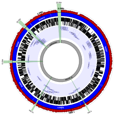
scaffolds-and-genes-plus-contig-list.txt:
# percent-GC graph with coordinates overlaid
%GC0-100 graph-min=40,graph-max=70,no-labels=1
coords label-interval=1000000,innerf=same

contigs c1
# show assembly gaps as light lines on the blue scaffolds
new ag rectangle innerf=same,outerf=same,feat-type=assembly_gap,color1=white,color2=white,stroke-width=2.5,opacity=0.7
# label each scaffold with its accession number
medium-label innerf=same+0.01,label-function=primary_id,feat-track=c1,text-color=white,packer=none,font-weight=bold
tiny-cgap

# invisible tRNAs
small-cgap
tRNAs trnas heightf=0.01,color1=none,color2=none

genes-fwd
genes-rev
small-cgap

# link back to invisible tRNAs from a few tracks before
new r1 rectangle heightf=0.01,color1=#eaeaff,color2=#eaeaff
new r2 rectangle heightf=0.2,color1=#eaeaff,color2=#eaeaff
large-label heightf=0.2,outerf=same,feat-track=trnas,style=signpost,label-function=product,draw-link=1,color1=#d0d0f0,color2=#7070f0,link-color=#7070f0,stroke-width=1.5,font-width-frac=3.5
new r3 rectangle heightf=0.01,color1=#eaeaff,color2=#eaeaff

# display 'genome' feature from contig_list file
new gr1 rectangle outerf=0.4,heightf=0.05,feat-type=genome,color1=#a0a0a0,color2=#000000,stroke-width=2
medium-label grl1 innerf=same,label-function=primary_id,feat-track=gr1,font-weight=bold

# highlight gaps between scaffolds/contigs
new cg1 rectangle innerf=same,outerf=1.1,feat-type=contig_gap,opacity=0.3,color1=green,color2=darkgreen,stroke-width=2
medium-label cgl1 innerf=1.1,feat-track=cg1,label-function=length_kb
This configuration file is almost identical to the previous one. The
only differences are that we’ve removed the lines responsible for
drawing the figure caption in the center of circle, and have added
about 7 new lines at the end. The first of those lines (see below)
draw and label the genome features that were created because of the
corresponding genome lines in the input contig file. They appear as
the grey curved rectangles in the middle. For demonstration purposes
we’ve labeled Scfld12 as “unknown” (in the contig list file, not the
config. file) even though it’s also a sequence from P. acnes
# display 'genome' feature from contig_list file
new gr1 rectangle outerf=0.4,heightf=0.05,feat-type=genome,color1=#a0a0a0,color2=#000000,stroke-width=2
medium-label grl1 innerf=same,label-function=primary_id,feat-track=gr1,font-weight=bold
The last 3 lines highlight the newly-created contig_gap features in
green and use the length_kb label function to automatically label
each one with its length. As you can see in the figure, these
contig_gaps correspond exactly to what was specified in the
contig_list file.
# highlight gaps between scaffolds/contigs
new cg1 rectangle innerf=same,outerf=1.1,feat-type=contig_gap,opacity=0.3,color1=green,color2=darkgreen,stroke-width=2
medium-label cgl1 innerf=1.1,feat-track=cg1,label-function=length_kb
