Displaying SNPs and indels

In this tutorial we’ll cover using Circleator to display SNPs and indels between closely-related strains. Before proceeding with the tutorial, please make sure that you have Circleator installed as described in the Circleator Installation Guide.

Outline

Example 1: Reading single-sample variants from VCF files

Reading single-sample variants from VCF files

Download the input and configuration files

In this first example we’ll look at displaying variants (SNPs, insertions, and deletions) from VCF files. We’re going to use the same reference genome, that of Enterobacteria phage lambda, as in Examples 1 and 2 from the Coverage Plots tutorial. In that tutorial we used Bowtie2 to align the synthetic read data provided with Bowtie against the phage lambda genome, as described in the Bowtie2 documentation. The Bowtie2 documentation also describes how to call variants and generate a VCF file with the samtools package and one of the BAM alignment files. We’ll use that VCF file for our first Circleator example. There’s just one small difference between the samtools command in the Bowtie documentation and the one that we’re going to use, because we want to generate a “.vcf” file rather than a “.bcf” file (i.e., a plain VCF file rather than a binary-encoded VCF file.) So instead of the following command, from the Bowtie2 documentation:

samtools mpileup -uf lambda_virus.fa eg2.sorted.bam | bcftools view -bvcg - > eg2.raw.bcf

We will instead use this command (with no -b flag and “.vcf” instead of “.bcf”):

samtools mpileup -uf lambda_virus.fa eg2.sorted.bam | bcftools view -vcg - > eg2.raw.vcf

Here is the VCF file that this command should produce, assuming that it’s run on the eg2.sorted.bam file from the Coverage Plots tutorial:

eg2.raw.vcf

Here is the GenBank flat file for the phage lambda genome:

NC_001416.1.gb

Here is the contig list file that reads the GenBank flat file but which tells Circleator to use “gi|9626243|ref|NC_001416.1|” as the id for the sequence that it contains, instead of “NC_001416”. This file is passed to Circleator’s --contig_list option, rather than passing the GenBank flat file directly to the --data option. Without this indirection Circleator won’t be able to match the variants in the VCF file (which are looking for a sequence with id “gi|9626243|ref|NC_001416.1|”, not “NC_001416”) with the reference sequence. This id-matching issue is also described in the Coverage Plots tutorial.

contig-list-ex1-gb.txt

And here is the Circleator configuration file for our first figure:

variants-ex1.txt

Run Circleator

Once you’ve downloaded or generated the necessary files, you’re ready to run Circleator, like so:

$ circleator --contig_list=contig-list-ex1-gb.txt --config=variants-ex1.txt > variants-ex1.svg

Convert the figure from SVG to PNG

If everything looks good so far then use rasterize-svg to convert the SVG to a PNG file:

$ rasterize-svg variants-ex1.svg png 3000 3000

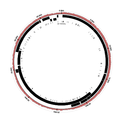
Here’s what the result should look like:

variants-ex1.png
(data: NC_001416.1.gb config: variants-ex1.txt, full size PNG | SVG)

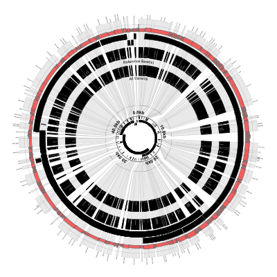
Blow things up

This type of figure is useful for visualizing where the SNPs and indels tend to cluster, but does not provide as much detail as the VCF file. One thing we can do is “blow up” or expand the variant loci (i.e., manipulate the scale of the figure around the circumference of the circle so that the regions of interest are expanded or stretched and all the other regions are compressed accordingly.) We can do this with the scaled-segment-list glyph in Circleator and, once the scale has been changed, we will have more space to overlay useful information on the variant loci. We’ll use the same input contig list file, GenBank flat file, and VCF file, but the following modified Circleator configuration file:

variants-ex1b.txt

Save the above file and rerun Circleator, replacing the original configuration file with the new one (and changing the name of the output SVG and PNG files):

$ circleator --contig_list=contig-list-ex1-gb.txt --config=variants-ex1b.txt > variants-ex1b.svg
$ rasterize-svg variants-ex1b.svg png 3000 3000

variants-ex1b.png
(data: NC_001416.1.gb config: variants-ex1b.txt, full size PNG | SVG)

In this version of the figure, notice that:

Each variant locus is shaded grey and expanded by about 100X
The coordinate labels have been relocated to the inside of the figure
The reference and variant base(s) are now overlaid on the figure
Each variant locus is labeled with its base position (the outermost part of the figure)
The small inner circle shows the genes and SNPs without any scaling
Some of the called variants overlap (e.g., position 12580-12585)