
Gene Conservation Visualization
In this tutorial we’ll show how to use Circleator to visualize patterns of gene conservation in two or more closely-related bacterial strains or serovars. Before proceeding with this tutorial, please make sure that you have Circleator installed as described in the Circleator Installation Guide.
Outline
-
Example 1: BLAST Score Ratio (BSR) Output
Example 1: BLAST Score Ratio (BSR) Output
The BLAST Score Ratio (BSR) Analysis Tool is a method and tool for normalizing raw BLAST scores in order to visualize the degree of proteome similarity between three genomes. Circleator can parse output from the BSR Analysis Tool and, although the tool itself is limited to 3-way comparisons, Circleator can combine output from multiple 3-way BSR runs (with a query genome in common) to visualize comparisons of arbitrary numbers of genomes.
We’ll start by drawing a Circleator figure for the BSR output from the test files distributed with the tool (the “TEST FILES” link on the BSR home page.) This example is a comparison of the following 3 genomes:
- Chlamydophila caviae GPIC (NC_003361.3)
- Chlamydia muridarum Nigg (NC_002620.2)
- Chlamydophila pneumoniae AR39 (NC_002179.2)
Download the input and configuration files
To draw the figure we’ll need the following input files:
- The GenBank flat file for our reference genome, Chlamydophila caviae GPIC: NC_003361.3.gbk
- The main BSR output file: Cc_GPIC_Cm_Nigg_Cp_AR39.txt
- A Circleator configuration file: bsr-1.txt
Run Circleator
Now that we have an input annotation file, the BSR output, and a Circleator configuration file, all that remains is to run Circleator, like so:
$ circleator --data=NC_003361.3.gbk --config=bsr-1.txt > bsr-1.svg
Convert the figure from SVG to PNG
Let’s convert the SVG image to PNG for viewing:
$ rasterize-svg bsr-1.svg png 3000 3000
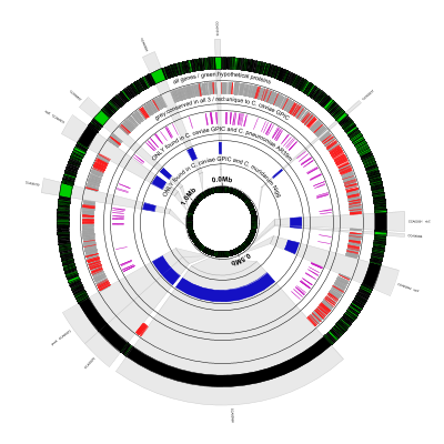
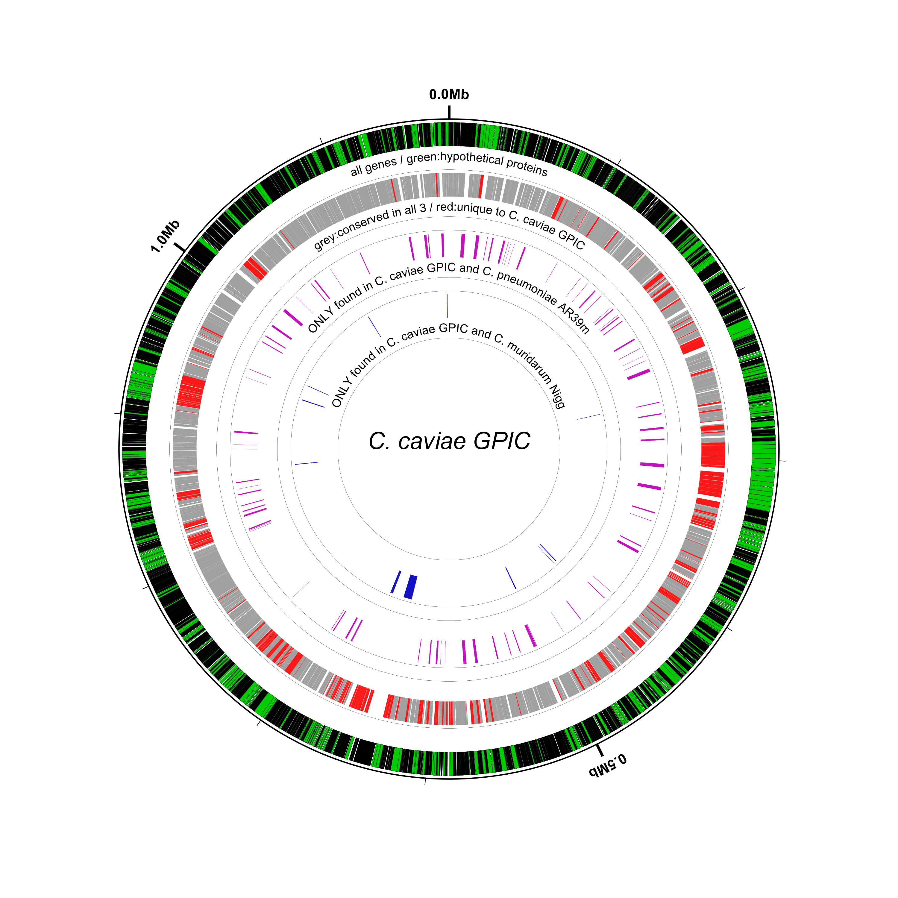
Here is the result:

There’s a lot going on in the configuration file for this figure, so let’s break it down a few lines at a time. The task of the first line is simply to read the BSR output file and assign aliases (“Cm” for Chlamydia muridarum Nigg and “Cp” for Chlamydophila pneumoniae AR39) to the two non-reference genomes used in the comparison:
# read BSR output and assign aliases to the two query genomes ("Cm", "Cp")
new load_bsr1 load-bsr heightf=0,bsr-file=./Cc_GPIC_Cm_Nigg_Cp_AR39.txt,genome1=Cm,genome2=Cp
The next couple of lines draw the labeled coordinate sequence axis (“0.0Mb”, etc.) followed by a very small gap:
# draw ruler/coordinates
coords

tiny-cgap
The next few lines are responsible for drawing the black and green outer circle. Black (curved) rectangles are drawn for every gene feature in the reference. Next, green rectangles are overlaid on top of the black ones to indicate which genes’ proteins are annotated as hypothetical. Here’s the line that draws all the genes in black (the default color):
genes
And here’s the line that overlays green on the hypotheticals. The options innerf=same and outerf=same tell Circleator
to place this track exactly over (i.e., on top of) the previous one. The feat-tag and feat-tag-regex options say to
look at the product feature tag and find any CDS features whose product matches the string “hypothetical protein”:
# highlight conserved hypotheticals
new HCH rectangle feat-type=CDS,feat-tag=product,feat-tag-regex=hypothetical\sprotein,innerf=same,outerf=same,opacity=0.8,color1=#00ff00
The next two lines print a label for the preceding track and then leave a small gap. Note the use of “ ” (the
HTML entity code for a non-breaking space) instead of a literal space character (“ “), because spaces are not allowed
in the options portion of a Circleator track definition:
medium-label label-text=all genes / green:hypothetical proteins
small-cgap
These lines draw a thin grey circle and leave a very small gap (the comment here refers to the next line that’s coming up):
# genes that are present in all 3 genomes
new CH1 rectangle color1=none,color2=#000000,heightf=0.14,feat-type=contig
tiny-cgap outerf=same
This next line draws genes conserved in all 3 genomes in grey. The crucial
options to pay attention to here are genomes=Cm|Cp and
signature=11. The first of these options lists the non-reference
genomes (using the aliases we defined earlier) on which we want to
filter, and the second of the options gives the filter to use, in
which “0” means “this strain must NOT be present” and “1” means “this
strain MUST be present.” “11” means to display only genes that are
conserved in both query genomes, Cm and Cp. Since conservation is
calculated relative to the reference we know that the gene is
conserved in the reference:
new bsr_all bsr 0.07 threshold=0.4,genomes=Cm|Cp,signature=11,color1=#a0a0a0,color2=#a0a0a0
Now we change the signature from “11” to “00” to find genes that are present in the reference, but NOT either of the query strains (i.e., genes that are unique to the reference at the given BSR similarity threshold.) These genes are colored green:
# genes that are unique to the reference
new bsr_ref bsr 0.07 threshold=0.4,genomes=Cm|Cp,signature=00,color1=#f91919,color2=#f91919,innerf=same
Label and gap:
medium-label label-text=grey:conserved in all 3 / red:unique to C. caviae GPIC
medium-cgap
Grey circle and gap:
# genes that are present only in the reference and Chlamydophila pneumoniae AR39
new CH1 rectangle color1=none,color2=#000000,heightf=0.14,feat-type=contig
tiny-cgap outerf=same
Now we’re showing genes that are present in the reference and Cp, but NOT Cm (i.e., signature=”01”):
new bsr_cp bsr 0.07 threshold=0.4,genomes=Cm|Cp,signature=01,color1=#c411be,color2=#c411be
Label and gap:
medium-label label-text=ONLY found in C. caviae GPIC and C. pneumoniae AR39m
medium-cgap
Grey circle and gap:
# genes that are present only in the reference and Chlamydia muridarum Nigg
new CH2 rectangle color1=none,color2=#000000,heightf=0.14,feat-type=contig
tiny-cgap outerf=same
Finally we’re showing genes that are present in the reference and CM, but NOT Cp (i.e., signature=”10”):
new bsr_cm bsr 0.07 threshold=0.4,genomes=Cm|Cp,signature=10,color1=#1511c4,color2=#1511c4
medium-label label-text=ONLY found in C. caviae GPIC and C. muridarum Nigg
Finally, we’re going to place a caption/figure title in the center of the image:
# caption
large-label innerf=0,label-text=C. caviae GPIC,label-type=horizontal,font-style=italic
Display which genes are conserved
This figure is interesting, but we’d really like to be able to see which genes are conserved. The
following configuration file uses the scaled-segment-list glyph to selectively expand (i.e., increase
the scale of) a subset of the genes, which gives us enough space in the figure to add the genes’
locus ids and, for those that have them, their gene symbols. Here’s the configuration file:
Using this configuration file, run Circleator again using the same reference data, but this time send the output to bsr-2.svg and then convert it to PNG format:
$ circleator --data=NC_003361.3.gbk --config=bsr-2.txt > bsr-2.svg
$ rasterize-svg bsr-2.svg png 3000 3000
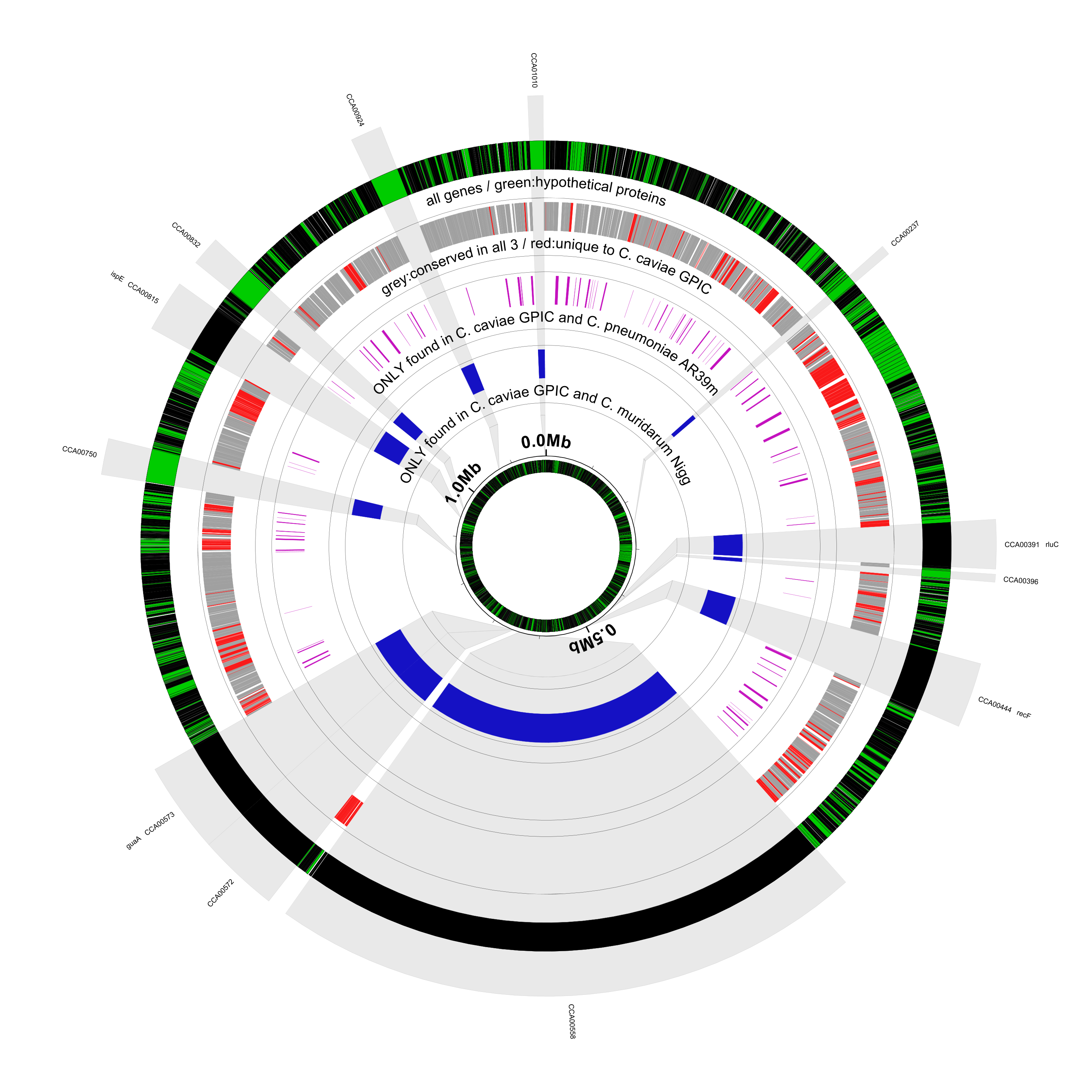
Comparing the output with the previous figure it’s obvious that the blue genes have been made significantly larger. It’s also now easy to see–by tracing the lines from the center out–which of those blue genes are annotated as “hypothetical protein”s in the reference. Finally, note that the scale markings around the outside of the circle (e.g., 0.0Mb, 0.5Mb, 1.0Mb) are no longer evenly spaced, thanks to the expansion of the sequence scale at the regions of interest (the blue genes):

Only a few lines were added to bsr-1.txt to get to bsr-2.txt and achieve this effect. First, we define the
sequence regions to be expanded, corresponding to all genes with a BSR signature of “10” i.e., genes that
are present in the reference and Cm but not Cp. Setting the height of this track to zero (the “0” in column
4) makes these features invisible so they don’t appear twice. Note that we’ve named this invisible
track containing the genes we’re interested in bsr_cm_d:
# expand each BSR region by 25X
new bsr_cm_d bsr 0 threshold=0.4,genomes=Cm|Cp,signature=10,color1=none,color2=none
Next we use the scaled-segment-list type to expand all the features from the previous track
(feat-track=bsr_cm_d) by a factor of 25 (scale=25). We’ve named this track ssl1:
new ssl1 scaled-segment-list feat-track=bsr_cm_d,scale=25
The next line shades each of the expanded regions grey. Since this track is drawn before any of the genes
or other annotation it won’t obscure them from view. Note that we’ve set feat-track=ssl1 to indicate
that the scaled-segment-list features should be expanded, but we could also have set feat-track=bsr_cm_d
and achieved the same result (because although the scaled segment features and the blue gene features
are different types of features they occupy the exact same set of sequence regions):
# highlight expanded regions
new hssl1 rectangle feat-track=ssl1,opacity=0.2,innerf=0,outerf=1.1,color1=#909090,color2=black
In the next two tracks we again refer back to the expanded features, this time using feat-track=bsr_cm_d,
in order to print the locus id (gene-function=locus) and gene symbol (gene-function=tag,tag-name=gene)
for each of the highlighted and expanded genes:
# label genes with locus and gene id
small-label lg1 innerf=1.12,label-function=locus,feat-track=bsr_cm_d,packer=none,label-type=spoke
small-label lg2 innerf=1.22,label-function=tag,tag-name=gene,feat-track=bsr_cm_d,packer=none,label-type=spoke
Finally, the following line in bsr-1.txt:
coords
had to be changed in bsr-2.txt. In particular, we set innerf=1.0 to reset the position of the coordinate labeling track
after drawing the gene locus ids and gene symbols around the outside of the image. If we had not made this
change then the sequence coordinate labels would appear immediately inside the previous track (the gene symbol labels,
which aren’t where we want the coordinate labels to be):
coords innerf=1.0
Add unscaled inner circle
Abrupt scale changes can be somewhat confusing and disorienting. One way to ameliorate the problem is to display an unscaled representation of the reference sequence in the middle of the figure and then use shading to depict the expansion of scale at the loci of interest. In this next figure we’ve made some slight modifications to do just that. The configuration file for the new figure is here:
Rerun Circleator and the rasterizer with the new configuration file:
$ circleator --data=NC_003361.3.gbk --config=bsr-3.txt > bsr-3.svg
$ rasterize-svg bsr-3.svg png 3000 3000
Here’s what the result looks like:
And here are the differences (as reported by the Linux diff command) between bsr-2.txt and bsr-3.txt, along with
some commentary. Note that lines beginning with < show what’s in the original configuration file, bsr-2.txt,
whereas those that start with > show the corresponding line(s) in bsr-3.txt.
diff bsr-2.txt bsr-3.txt
8c8
The shaded highlights for the expanded genes/regions used to go all the way to the center (innerf=0) but
we’ve changed them to stop at (radial) position 0.32 (innerf=0.32):
< new hssl1 rectangle feat-track=ssl1,opacity=0.2,innerf=0,outerf=1.1,color1=#909090,color2=black
---
> new hssl1 rectangle feat-track=ssl1,opacity=0.2,innerf=0.32,outerf=1.1,color1=#909090,color2=black
The outer set of coordinate labels have been removed. This means that the next track, tiny-cgap is now
responsible for resetting the track position after drawing the gene locus ids and gene symbols:
14,17c14
< # draw ruler/coordinates
< coords innerf=1.0
<
< tiny-cgap
---
> tiny-cgap outerf=1.0
We’ve removed the figure caption in the center to make room for the inner unscaled circle:
46,47c43,57
< # caption
< large-label innerf=0,label-text=C. caviae GPIC,label-type=horizontal,font-style=italic
---
This line connects the scaled highlight features with the unscaled inner ring. Note the use of outer-scale
and inner-scale to indicate that the sequence scale is being changed as we move from position 0.32 (outerf)
to position 0.22 (innerf). outer-scale=default means that the scale on the outer edge of this track
matches whatever scale is already in place (i.e., the one where the blue genes are expanded) and inner-scale=none
means that the scale on the inner edge of this track should be normal/unscaled. Circleator performs a linear
interpolation between the two scales/coordinate systems, which results in the effect seen in the figure,
connecting the large/scaled highlight regions to the small/unscaled inner circle:
> # connect outer scaled circle to inner unscaled circle
> new hssl2 rectangle innerf=0.22,outerf=0.32,feat-track=ssl1,opacity=0.2,color1=#909090,color2=black,stroke-width=1,inner-scale=none,outer-scale=default
>
In the previous line/track we changed the scale using inner-scale. However, this only affects the scale/coordinate
system for that one track. In order to change the coordinate system back to normal for the remainder of the figure,
we use the following line. feat-type=dummy specifies a feature type that does not exist, so no scaling is applied.
Any time a scaled-segment-list track appears it replaces whatever scaling was previously in place, so this line
resets the scale to normal:
> # restore unscaled coordinates
> new SSLR scaled-segment-list scale=1,feat-type=dummy
>
Now that the scale has been reset to normal we can draw a small coordinate circle, followed by just the gene/ hypothetical gene track. We could have included more, but we are starting to run out of space here:
> # inner (unscaled) circle
> coords innerf=0.22,heightf=0.008
> tiny-cgap
>
> # repeat all genes/hypotheticals track
> genes heightf=0.03
> # highlight conserved hypotheticals
> new HCH rectangle feat-type=CDS,feat-tag=product,feat-tag-regex=hypothetical\sprotein,innerf=same,outerf=same,opacity=0.8,color1=#00ff00
>
